Quantum Optics II Two-level system
fengxiaot Lv4

A two-level system is the simplest quantum model that still captures the essential features of light-matter interaction. By focusing on just two states and the coupling between them, it explains many key phenomena in quantum optics, including Rabi oscillations, dressed states, and Autler–Townes splitting.

Two-level System

Basic

The Hamiltonian of a two-level system is[1]

H=H0+WH = H_0 + W

Let {∣φ1⟩,∣φ2⟩}\{\ket{\varphi_1},\ket{\varphi_2}\} be the eigenstates of H0H_0 with eigenvalues E1,E2E_1,E_2, which forms the basis of state space. Suppose that WW has purely non-diagonal matrix elements, which describes the interaction between the two levels. The matrix representation of HH is then

H=[E1W12W21E2]H = \begin{bmatrix} E_1 & W_{12} \\ W_{21} & E_2 \end{bmatrix}

where W12=W21∗W_{12} = W_{21}^*. Diagonalize the matrix HH, we can find the following eigenvalues

E+=12(E1+E2)+12(E1−E2)2+4∣W12∣2E_+ = \frac{1}{2} (E_1 + E_2) + \frac{1}{2} \sqrt{(E_1 - E_2 )^2 + 4 |W_{12}|^2}

E−=12(E1+E2)−12(E1−E2)2+4∣W12∣2E_- = \frac{1}{2} (E_1 + E_2) - \frac{1}{2} \sqrt{(E_1 - E_2 )^2 + 4 |W_{12}|^2}

Introducing two parameters

Em=12(E1+E2),Δ=12(E1−E2)E_m = \frac{1}{2} (E_1 + E_2),\quad \Delta = \frac{1}{2}(E_1 - E_2)

The eigenvalues can be written as

E+=Em+Δ2+∣W12∣2,E−=Em−Δ2+∣W12∣2E_+ = E_m + \sqrt{\Delta^2 + |W_{12}|^2},\quad E_- = E_m -\sqrt{\Delta^2 + |W_{12}|^2}

The corresponding eigenvectors (not normalized) are

∣+⟩=Δ−Δ2+∣W12∣2W12∣φ0⟩+∣φ1⟩,∣−⟩=Δ+Δ2+∣W12∣2W12∣φ0⟩+∣φ1⟩\ket{\mathrm{+}} = \frac{\Delta-\sqrt{\Delta^2 + |W_{12}|^2}}{W_{12}} \ket{\varphi_0} + \ket{\varphi_1},\quad \ket{\mathrm{-}} = \frac{\Delta+\sqrt{\Delta^2 + |W_{12}|^2}}{W_{12}} \ket{\varphi_0} + \ket{\varphi_1}

Dynamics

Assume that the system was initially in the state ∣ψ(0)⟩=∣φ1⟩\ket{\psi(0)} = \ket{\varphi_1} at t=0t=0 . The probability to find the system in the state ∣φ2⟩\ket{\varphi_2} at time tt is

P12(t)=⟨φ2∣ψ(t)⟩=∣W12∣2∣W12∣2+Δ2sin⁡2(∣W12∣2+Δ2tℏ)=∣W12∣2∣W12∣2+Δ2sin⁡2(E+−E−2ℏt)\mathcal{P}_{12}(t) = \braket{\varphi_2|\psi(t)} =\frac{|W_{12}|^2}{|W_{12}|^2+\Delta^2} \sin^2 \left(\sqrt{|W_{12}|^2+\Delta^2} \frac{t}{\hbar}\right) = \frac{|W_{12}|^2}{|W_{12}|^2+\Delta^2} \sin^2 \left(\frac{E_+ - E_-}{2 \hbar} t\right)

This expression shows that the probability P12(t)\mathcal{P}_{12}(t) oscillates over time with a frequency of Ω=∣W12∣2+Δ2/ℏ=(E+−E−)/2ℏ\Omega = \sqrt{|W_{12}|^2+\Delta^2} / \hbar = (E_+ - E_-) / 2 \hbar and an amplitude of ∣W12∣2∣W12∣2+Δ2\frac{|W_{12}|^2}{|W_{12}|^2+\Delta^2}.

/* Note: If E1=E2E_1 = E_2, which means Δ=0\Delta = 0, the amplitute of oscilation will be 11. There exists some certain times when all particles transmit from ∣φ1⟩\ket{\varphi_1} to ∣φ2⟩\ket{\varphi_2}. */


Dipole Interaction

Atom Field Interaction

We begin our treatment with a general description of the atom-field interaction[2]. We will assume the field is monochromatic and linear polarized with angular frequency ω\omega

E=E0cos⁡ωt e^\boldsymbol{E} = E_0 \cos \omega t \,\hat{\mathbf{e}}

Here, e^\hat{e} is the unit polarization vector of the field.

/* Note: We are ignoring the spatial dependence of the field, only writing down the field at the location of the atom. This is appropriate in the dipole approximation or long-wavelength approximation, where we assume that the wavelength of the field is much longer than the size of the atom, so that we can neglect any variations of the field over the extent of the atom. */

The atomic free-evolution Hamiltonian is given by

Hatom=12ℏω0σzH_\text{atom} = \frac{1}{2} \hbar \omega_0 \sigma_z

The atom-field interaction Hamiltonian is

Hint=−D⋅EH_\text{int} = - \boldsymbol{D} \cdot \boldsymbol{E}

where D=−eR\boldsymbol{D} = -e \boldsymbol{R} is the electric dipole moment of an atom, R\boldsymbol{R} is the position vector pointing from the nuclei to the electron. Using parity, we can easily prove that ⟨g∣D∣g⟩=⟨e∣D∣e⟩=0\braket{g|\boldsymbol{D}|g} = \braket{e|\boldsymbol{D}|e} = 0. Therefore, in the two dimensional state space, the dipole moment operator can be decomposed into

D=⟨g∣D∣e⟩∣g⟩⟨e∣+⟨e∣D∣g⟩∣e⟩⟨g∣\boldsymbol{D} = \braket{g|\boldsymbol{D}|e} \ket{g}\bra{e} + \braket{e|\boldsymbol{D}|g} \ket{e}\bra{g}

We can choose the phase of the dipole matrix element ⟨g∣D∣e⟩\braket{g|\boldsymbol{D}|e} such that it is real (using Clebsch-Gordan), in which case the expression we can write the dipole moment operator as

D=⟨g∣D∣e⟩(σ†+σ)\boldsymbol{D} = \braket{g|\boldsymbol{D}|e} (\sigma^\dagger + \sigma)

The atom-field interaction Hamiltonian becomes

Hint=−⟨g∣D⋅e^∣e⟩E0(σ†+σ)cos⁡ωtH_\text{int} = -\braket{g|\boldsymbol{D}\cdot \hat{\mathbf{e}} |e}E_0 (\sigma^\dagger + \sigma) \cos \omega t

Defining Rabi frequency Ω0=−⟨g∣D⋅e^∣e⟩E0/ℏ\Omega_0 = -\braket{g|\boldsymbol{D}\cdot \hat{\mathbf{e}} |e}E_0/\hbar, the Hamiltonian now becomes

Hint=ℏΩ0cos⁡ωt (σ†+σ)=ℏΩ02(σ†+σ)(eiωt+e−iωt)H_\text{int} = \hbar \Omega_0 \cos\omega t\, (\sigma^\dagger + \sigma) = \frac{\hbar \Omega_0}{2} (\sigma^\dagger + \sigma)(\mathrm{e}^{\mathrm{i}\omega t} + \mathrm{e}^{-\mathrm{i}\omega t})

The total Hamiltonian is

H=Hatom+Hint=12ℏω0σz+ℏΩ02(eiωt+e−iωt)(σ†+σ)H = H_\text{atom} + H_\text{int} = \frac{1}{2} \hbar \omega_0 \sigma_z + \frac{\hbar \Omega_0}{2} (\mathrm{e}^{\mathrm{i}\omega t} + \mathrm{e}^{-\mathrm{i}\omega t}) (\sigma^\dagger + \sigma)

where σ†\sigma^\dagger is the raising operator ∣e⟩⟨g∣\ket{e}\bra{g} and σ\sigma is the lowering operator ∣g⟩⟨e∣\ket{g}\bra{e}, σx=σ†+σ\sigma_x = \sigma^\dagger + \sigma.

Rabi Oscillation

The Hamiltonian of a two-level system is

H=12ℏω0σz+12ℏΩ0(eiωt+e−iωt)(σ†+σ)H = \frac{1}{2} \hbar \omega_0 \sigma_z + \frac{1}{2}\hbar \Omega_0 (\mathrm{e}^{\mathrm{i}\omega t} + \mathrm{e}^{-\mathrm{i}\omega t}) (\sigma^\dagger + \sigma)

Performing the following rotating frame transformation

U=exp⁡(i2ωtσz)U=\exp \left( \frac{\mathrm{i}}{2} \omega t \sigma_z \right)

The Hamiltonian in the rotating frame will become

H~=UHU†+iℏU˙U†=−12ℏδσz+12ℏΩ0σ†(1+ei2ωt)+12ℏΩ0σ(1+e−i2ωt)\tilde{H} = UHU^\dagger+\mathrm{i}\hbar \dot{U} U^\dagger = -\frac{1}{2}\hbar\delta \sigma_z + \frac{1}{2} \hbar \Omega_0 \sigma^\dagger (1+ \mathrm{e}^{\mathrm{i} 2\omega t}) + \frac{1}{2} \hbar \Omega_0 \sigma (1+ \mathrm{e}^{-\mathrm{i} 2\omega t})

where δ:=ω−ω0\delta := \omega - \omega_0 is the detuning of laser frequency. Since ei2ωt\mathrm{e}^{\mathrm{i} 2\omega t} and e−i2ωt\mathrm{e}^{-\mathrm{i} 2\omega t} are rapid oscillating terms, we can omit them. This is called rotating-wave approximation (RWA). RWA requires ∣ω0−ω∣≪ω0+ω|\omega_0 - \omega| \ll \omega_0 +\omega. In this case, the Hamiltonian becomes

H~RWA=−12ℏδσz+12ℏΩ0(σ†+σ)\tilde{H}_\text{RWA} = -\frac{1}{2}\hbar\delta \sigma_z + \frac{1}{2} \hbar \Omega_0 (\sigma^\dagger + \sigma)

We can actually make the rotating-wave approximation from the very beginning. The electric field and the dipole moment can be decomposed into the positive-frequency part and the negative frequency part:

E=E++E−=E02e−iωt e^+E02eiωt e^\boldsymbol{E} = \boldsymbol{E}^+ +\boldsymbol{E}^- = \frac{E_0}{2} \mathrm{e}^{-\mathrm{i}\omega t}\,\hat{\mathbf{e}} + \frac{E_0}{2} \mathrm{e}^{\mathrm{i}\omega t}\,\hat{\mathbf{e}}

D=D++D−=⟨g∣D∣e⟩σ+⟨g∣D∣e⟩σ†\boldsymbol{D} = \boldsymbol{D}^+ + \boldsymbol{D}^- = \braket{g|\boldsymbol{D}|e} \sigma + \braket{g|\boldsymbol{D}|e} \sigma^\dagger

Only E+⋅D−\boldsymbol{E}^+ \cdot \boldsymbol{D}^- and E−⋅D+\boldsymbol{E}^- \cdot \boldsymbol{D}^+ are on-resonant, which means the effective terms in the Hamiltonian remain

HRWA=12ℏω0σz+12ℏΩ0(σ†e−iωt+σeiωt)H_\text{RWA} = \frac{1}{2} \hbar \omega_0 \sigma_z + \frac{1}{2}\hbar \Omega_0 (\sigma^\dagger \mathrm{e}^{-\mathrm{i}\omega t}+\sigma\mathrm{e}^{\mathrm{i}\omega t})

If we directly perform rotating frame transformation on HRWAH_\text{RWA}, we will immediately get

H~RWA=−12ℏδσz+12ℏΩ0(σ†+σ)\tilde{H}_\text{RWA} = -\frac{1}{2}\hbar\delta \sigma_z + \frac{1}{2} \hbar \Omega_0 (\sigma^\dagger + \sigma)

We find that the Hamiltonian in the rotating frame H~\tilde{H} is time-independent, which enables us to use time evolution operator to depict the evolved state at any time

H~=−12ℏδσz+12ℏΩ0(σ†+σ)=[−12ℏδ12ℏΩ012ℏΩ012ℏδ]\tilde{H} = -\frac{1}{2}\hbar\delta \sigma_z + \frac{1}{2} \hbar \Omega_0 (\sigma^\dagger + \sigma) = \begin{bmatrix} -\frac{1}{2}\hbar \delta & \frac{1}{2}\hbar \Omega_0 \\ \frac{1}{2}\hbar \Omega_0 & \frac{1}{2}\hbar \delta \end{bmatrix}

U~=exp⁡(−iℏH~t)=[cos⁡Ωt2+iδΩsin⁡Ωt2−isin⁡Ωt2Ω0Ω−isin⁡Ωt2Ω0Ωcos⁡Ωt2−iδΩsin⁡Ωt2]\tilde{U} = \exp\left( - \frac{\mathrm{i}}{\hbar} \tilde{H} t\right) = \begin{bmatrix} \cos\frac{\Omega t}{2} + \mathrm{i} \frac{\delta}{\Omega} \sin\frac{\Omega t}{2} & -\mathrm{i} \sin\frac{\Omega t}{2} \frac{\Omega_0}{\Omega} \\ -\mathrm{i} \sin\frac{\Omega t}{2} \frac{\Omega_0}{\Omega} & \cos\frac{\Omega t}{2} - \mathrm{i} \frac{\delta}{\Omega} \sin\frac{\Omega t}{2} \end{bmatrix}

For an atom initialized in the ground state ∣g⟩\ket{g}, the final state in the rotating frame is

∣ψ~(t)⟩=U~∣ψ~(0)⟩=U~∣g⟩\ket{\tilde{\psi}(t)} = \tilde{U} \ket{\tilde{\psi}(0)} = \tilde{U} \ket{g}

switching back to the lab frame (Schrödinger picture)

∣ψ(t)⟩=e−i2ωtσz∣ψ~(t)⟩=e−i2ωtσzU~∣g⟩=[−isin⁡Ωt2Ω0Ωe−i2ωtei2ωt(cos⁡Ωt2−iδΩsin⁡Ωt2)]\ket{\psi(t)} = \mathrm{e}^{-\frac{\mathrm{i}}{2}\omega t\sigma_z} \ket{\tilde{\psi}(t)} = \mathrm{e}^{-\frac{\mathrm{i}}{2}\omega t\sigma_z} \tilde{U} \ket{g} = \begin{bmatrix} -\mathrm{i} \sin\frac{\Omega t}{2} \frac{\Omega_0}{\Omega} \mathrm{e}^{-\frac{\mathrm{i}}{2}\omega t} \\ \mathrm{e}^{\frac{\mathrm{i}}{2}\omega t} \left( \cos\frac{\Omega t}{2} - \mathrm{i} \frac{\delta}{\Omega} \sin\frac{\Omega t}{2} \right) \end{bmatrix}

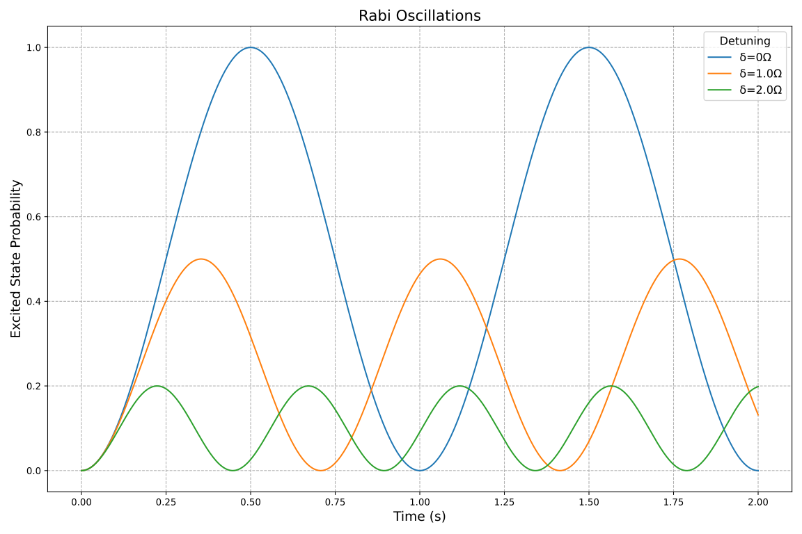
where Ω=Ω02+δ2\Omega = \sqrt{\Omega_0^2 + \delta^2} is called the generalized Rabi frequency. The probability to find the atom in the excited state at time tt is

∣⟨e∣ψ(t)⟩∣2=Ω02Ω2sin⁡2Ωt2=Ω02Ω02+Δ2sin⁡2Ω02+Δ2t2|\langle e| \psi(t)\rangle|^2 = \frac{\Omega_0^2}{\Omega^2} \sin^2\frac{\Omega t}{2} = \frac{\Omega_0^2}{\Omega_0^2+\Delta^2} \sin^2\frac{\sqrt{\Omega_0^2+\Delta^2} t}{2}

Dressed State

As long as we continuously shining the laser on the atom, the atom and the electric field can keep interacting and form a stable coupled system. The atom-field as a whole is now fully described by H~\tilde{H}. By diagonalizing H~\tilde{H}, we can find the new eigenenergies and eigenstates, which are so-called dressed states.

Still start with

H~=−12ℏδσz+12ℏΩ0σx=ℏ[−δ/2Ω0/2Ω0/2δ/2]\tilde{H} = -\frac{1}{2}\hbar\delta \sigma_z + \frac{1}{2} \hbar \Omega_0 \sigma_x = \hbar \begin{bmatrix} -\delta/2 & \Omega_0/2 \\ \Omega_0/2 & \delta/2 \end{bmatrix}

Diagonalize it we get

E+=ℏ2Ω02+δ2=ℏΩ2,∣+⟩=[cos⁡(θ/2)sin⁡(θ/2)]E_+ = \frac{\hbar}{2}\sqrt{\Omega_0^2+\delta^2}= \frac{\hbar\Omega}{2},\quad\ket{+}=\begin{bmatrix} \cos(\theta/2)\\ \sin(\theta/2) \end{bmatrix}

E−=−ℏ2Ω02+δ2=−ℏΩ2,∣−⟩=[−sin⁡(θ/2)cos⁡(θ/2)]E_- = -\frac{\hbar}{2}\sqrt{\Omega_0^2+\delta^2}= -\frac{\hbar\Omega}{2} ,\quad \ket{-}=\begin{bmatrix} -\sin(\theta/2) \\ \cos(\theta/2) \end{bmatrix}

in which tan⁡θ=−Ω0/δ,0≤θ<π\tan \theta = -\Omega_0/\delta ,0\le\theta < \pi is called the Stückelberg angle, Ω=Ω02+δ2\Omega = \sqrt{\Omega_0^2+\delta^2} is the generalized Rabi frequency.

/* Note: The sign convention and domain of Stückelberg angle are important! */

Free-evolution

When there is no external light field, the energy levels of the ground state and the excited state (in the rotating frame) are

Ee=−ℏδ2,Eg=ℏδ2E_e = -\frac{\hbar\delta}{2},\quad E_g = \frac{\hbar\delta}{2}

which coincides with the classical occasion: angular frequency of rotation is changed and part of energy is removed.

On-resonance

When the laser is on-resonant, δ=0\delta = 0. The energy level of dressed states are

E+=12ℏΩ0,E−=−12ℏΩ0E_+ = \frac{1}{2}\hbar\Omega_0,\quad E_- =-\frac{1}{2}\hbar\Omega_0

Meanwhile, θ=π/2\theta = \pi/2, thus

∣+⟩=12(∣e⟩+∣g⟩),∣−⟩=12(∣e⟩−∣g⟩)\ket{+} = \frac{1}{\sqrt{2}} (\ket{e}+\ket{g}),\quad \ket{-} = \frac{1}{\sqrt{2}} (\ket{e}-\ket{g})

Far-off-resonance

For large detuning ∣δ∣≫Ω0|\delta| \gg \Omega_0, we have[3]

  • δ<0\delta < 0, red detuned, θ→0\theta \to 0, ∣+⟩=∣e⟩\ket{+} = \ket{e} and ∣−⟩=∣g⟩\ket{-}=\ket{g}, thus

    E+=Ee≈−ℏδ2−ℏΩ024δ,E−=Eg≈ℏδ2+ℏΩ024δE_+ = E_e \approx -\frac{\hbar \delta}{2} - \frac{\hbar \Omega_0^2}{4\delta},\quad E_- =E_g \approx \frac{\hbar\delta}{2} + \frac{\hbar \Omega_0^2}{4\delta}

  • δ>0\delta >0, blue detuned, θ→π\theta \to \pi, ∣+⟩=∣g⟩\ket{+} = \ket{g} and ∣−⟩=−∣e⟩\ket{-}= -\ket{e}, thus

    E+=Eg≈ℏδ2+ℏΩ024δ,E−=Ee≈−ℏδ2−ℏΩ024δE_+ = E_g \approx \frac{\hbar\delta}{2} + \frac{\hbar \Omega_0^2}{4\delta},\quad E_- = E_e \approx -\frac{\hbar \delta}{2} - \frac{\hbar \Omega_0^2}{4\delta}

We can conclude that, when the detuning reverses its sign, although the mapping between ∣+⟩,∣−⟩\ket{+},\ket{-} and ∣e⟩,∣g⟩\ket{e},\ket{g} is swapped, the expressions for the corrected energy level of the ground state and the excited state remain unchanged.

Moreover, we find a unified energy shift formula for ground states

ΔEg=ℏΩ024δ\Delta E_g = \frac{\hbar \Omega_0^2}{4\delta}

This is crucial for building an optical dipole trap.

Autler-Townes Doublet

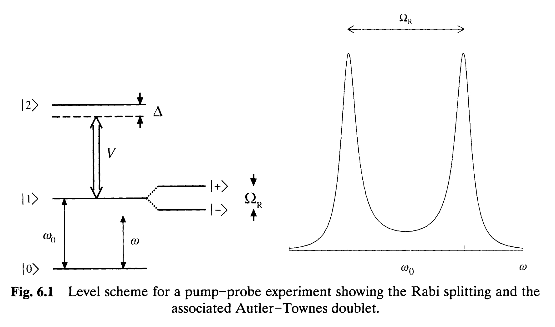
Consider a three-level atom with bare states ∣0⟩,∣1⟩\ket{0},\ket{1} and ∣2⟩\ket{2}. State ∣1⟩,∣2⟩\ket{1}, \ket{2} are strongly driven by a near-resonant laser[4]. As a result, the energy of the upper level ∣2⟩\ket{2} is pulled down by the light field, and the atom and field as a whole form two new dressed states ∣+⟩,∣−⟩\ket{+}, \ket{-} with energy splitting Ω\Omega, replacing the old energy levels ∣1⟩\ket{1} and ∣2⟩\ket{2}.

Now we apply a second weaker laser to probe the transition between the state ∣0⟩\ket{0} and the state ∣1⟩\ket{1}. As the frequency of the probe laser is swept through resonance with the bare transition frequency ω0\omega_0, the absorption spectrum obtained exhibits two peaks separated by the generalized Rabi frequency Ω\Omega associated with transitions between the bare states ∣1⟩\ket{1} and ∣2⟩\ket{2}, as shown in the following figure. The positions of these peaks differ from the bare transition frequency ω0\omega_0 by ±Ω/2\pm\Omega/2. In other words, the weaker laser actually detected the transition of ∣0⟩↔∣+⟩\ket{0}\leftrightarrow\ket{+} and ∣0⟩↔∣−⟩\ket{0}\leftrightarrow\ket{-}!

In 1955, Autler and Townes showed the spectrum discussed above utilizing a microwave transition of the OCS molecule[5]. The corresponding doublet is called the Autler-Townes doublet, or the dynamic Stark splitting.


  1. Cohen-Tannoudji C, Diu B, Franck Laloë. Quantum Mechanics, Volume 1: Basic Concepts, Tools, and Applications[M]. 2. Wiley VCH, 2019: 411-422. ↩︎

  2. Daniel A. Steck, Quantum and Atom Optics, available online at http://steck.us/teaching (revision 0.16.2, 15 November 2024). ↩︎

  3. Grynberg, G., Aspect, A., & Fabre, C. (2010). Introduction to Quantum Optics: From the Semi-classical Approach to Quantized Light. Cambridge: Cambridge University Press. ↩︎

  4. Barnett S M, Radmore P M. Methods in Theoretical Quantum Optics[M]. Oxford University Press, 2002 :182-221. ↩︎

  5. Autler, S. H., & Townes, C. H. (1955). Stark Effect in Rapidly Varying Fields. Phys. Rev., 100(2), 703–722. https://doi.org/10.1103/PhysRev.100.703 ↩︎