Quantum Optics VIII Time Dependent Perturbation Theory
fengxiaot Lv4

In time-dependent perturbation theory, the primary goal is to determine the time evolution of a perturbed quantum system, with a particular focus on calculating transition probabilities and modeling the irreversible decay of probability in a small quantum system coupled to a much larger system. The interaction picture will be employed to discuss time-dependent perturbations.

Time Dependent Perturbation Theory

General Theory

Come back to Schrödinger picture. Suppose at t=0t=0 we works out the eigenstates ∣n⟩\ket{n} of H0H_0 . We are interested in two of them, ∣f⟩\ket{f} and ∣i⟩\ket{i} (initial state and final state in Schrödinger picture). After time tt , the states in the Schrödinger picture become

∣f,t⟩=e−iℏEft∣f⟩∣i,t⟩=e−iℏEit∣i⟩\ket{f,t} = \mathrm{e}^{-\frac{\mathrm{i}}{\hbar} E_f t} \ket{f} \qquad \ket{i,t} = \mathrm{e}^{-\frac{\mathrm{i}}{\hbar} E_i t} \ket{i}

The questions is, what the transition probability Pfi(t)\mathcal{P}_{fi}(t) is for a system initially in the state ∣i⟩\ket{i} at time t=t0t=t_0 (could be zero) evolving into the state ∣f,t⟩\ket{f,t} at time tt ? Using the evolution operator, we can derive

Pfi(t)=∣⟨f,t∣US(t,t0)∣i,t0⟩∣2=∣⟨f∣eiℏEftUS(t,t0)e−iℏEit0∣i⟩∣2=∣⟨f∣UI(t,t0)∣i⟩∣2\mathcal{P}_{fi}(t) = \left| \langle f,t| U^S(t,t_0) |i,t_0\rangle\right|^2 = \left| \langle f| \mathrm{e}^{\frac{\mathrm{i}}{\hbar} E_f t} U^S(t,t_0) \mathrm{e}^{-\frac{\mathrm{i}}{\hbar} E_i t_0} |i\rangle\right|^2 = \left| \langle f| U^I(t,t_0) |i\rangle\right|^2

According to the first order perturbation theory, that is, take the first order of the Dyson series, the transition probability is

Pfi(t)=∣⟨fS∣UI(t,t0)∣iS⟩∣2=∣⟨fS∣−iℏ∫t0tdt1 HintI(t1)∣iS⟩∣2=∣⟨fS∣−iℏ∫t0tdt1 eiℏH0St1HintS(t1)e−iℏH0St1∣iS⟩∣2=1ℏ2∣∫t0tdt1 eiℏ(Ef−Ei)t1⟨f∣HintS(t1)∣i⟩∣2\begin{aligned} \mathcal{P}_{fi}(t) &= \left| \langle f^S| U^I(t,t_0) |i^S\rangle\right|^2 \\ &= \left| \langle f^S| -\frac{\mathrm{i}}{\hbar} \int_{t_0}^t \mathrm{d} t_1\, H^I_\text{int}(t_1) |i^S\rangle\right|^2 \\ &= \left| \langle f^S| -\frac{\mathrm{i}}{\hbar} \int_{t_0}^t \mathrm{d} t_1\, \mathrm{e}^{\frac{\mathrm{i}}{\hbar} H_0^S t_1} H^S_\text{int}(t_1) \mathrm{e}^{-\frac{\mathrm{i}}{\hbar} H_0^S t_1} |i^S\rangle\right|^2 \\ &= \frac{1}{\hbar^2} \left| \int_{t_0}^t \mathrm{d} t_1\, \mathrm{e}^{\frac{\mathrm{i}}{\hbar} (E_f - E_i) t_1} \langle f| H^S_\text{int}(t_1) |i\rangle\right|^2 \end{aligned}

The superscripts SS indicating Schrödinger picture of kets ∣f⟩\ket{f} and ∣i⟩\ket{i} are omitted. Define ωfi=Ef−Eiℏ\omega_{fi} = \frac{E_f-E_i}{\hbar}, we obtain the final formula of first-order perturbation theory.

Notice, however, this approach is valid only if Pfi≪1\mathcal{P}_{fi} \ll 1.

Sinusoidal Perturbation

Suppose HintS(t)=Wsin⁡ωtH^S_\text{int}(t) = W \sin \omega t , where WW is a time independent observation operator. Then

Pfi(t;ω)=1ℏ2∣∫t0tdt′ eiωfit′sin⁡ωt′⟨f∣W∣i⟩∣2=∣⟨f∣W∣i⟩∣24ℏ2∣1−ei(ωfi+ω)Tωfi+ω+1−ei(ωfi−ω)Tωfi−ω∣2\mathcal{P}_{fi}(t;\omega) = \frac{1}{\hbar^2} \left| \int_{t_0}^t \mathrm{d} t^\prime \, \mathrm{e}^{\mathrm{i} \omega_{fi} t^\prime} \sin \omega t^\prime \langle f| W |i\rangle\right|^2 = \frac{|\langle f| W |i\rangle|^2}{4 \hbar^2} \left|\frac{1-\mathrm{e}^{\mathrm{i}(\omega_{fi}+\omega)T}}{\omega_{fi}+\omega} + \frac{1-\mathrm{e}^{\mathrm{i}(\omega_{fi}-\omega)T}}{\omega_{fi}-\omega}\right|^2

in which T=t−t0T=t-t_0 . Resonance requires ω≃ωfi\omega \simeq \omega_{fi}. We introduce rotating-wave approximation

∣1−ei(ωfi+ω)Tωfi+ω∣=∣sin⁡[(ωfi+ω)T/2](ωfi+ω)/2∣≃0\left|\frac{1-\mathrm{e}^{\mathrm{i}(\omega_{fi}+\omega)T}}{\omega_{fi}+\omega}\right| = \left|\frac{\sin [(\omega_{fi}+\omega)T/2]}{(\omega_{fi}+\omega)/2}\right| \simeq0

which means that anti-resonant term is negligible on average since it has large frequency (ωfi+ω≫ωfi−ω)(\omega_{fi}+\omega \gg \omega_{fi}-\omega) and oscillates fast within a time period TT. Therefore, the transition probability becomes

Pfi(t;ω)=∣⟨f∣W∣i⟩∣24ℏ2sin⁡2[(ωfi−ω)T/2][(ωfi−ω)/2]2\mathcal{P}_{fi}(t;\omega) = \frac{|\langle f| W |i\rangle|^2}{4 \hbar^2} \frac{\sin^2 [(\omega_{fi}-\omega)T/2]}{[(\omega_{fi}-\omega)/2]^2}

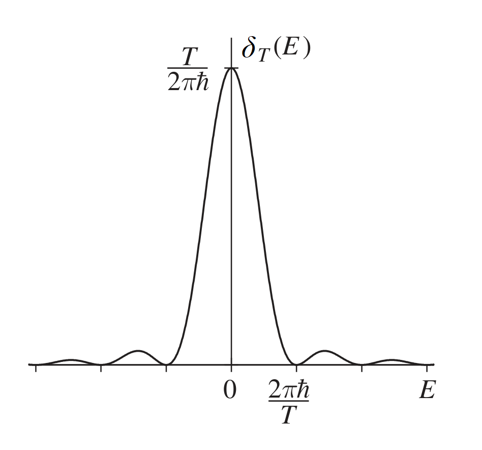
Notice that the sinc-squared function sequence Nπsin⁡2(Nx)(Nx)2\frac{N}{\pi} \frac{\sin^2 (Nx)}{(Nx)^2} approaches the behavior of delta function when N→∞N \to \infty. We naturally introduce a distribution δT(E)\delta_T(E) as follows

δT(E)=sin⁡2ET2ℏ(ET2ℏ)2T2πℏ=2ℏsin⁡2(ET/2ℏ)πTE2\delta_T(E) = \frac{\sin^2\frac{ET}{2\hbar}}{\left(\frac{ET}{2\hbar}\right)^2} \frac{T}{2\pi\hbar} = \frac{2\hbar \sin^2(ET/2\hbar)}{\pi T E^2}

which has the maximum value T2πℏ\frac{T}{2\pi \hbar} at E=0E=0 and its width of order is 2πℏT\frac{2\pi\hbar}{T}. It becomes delta function when T→∞T \to \infty. Therefore, the transition probability can be written as

Pfi(t;ω)=∣⟨f∣W∣i⟩∣2πT2ℏδT(Ef−Ei−ℏω)\mathcal{P}_{fi}(t;\omega) = |\langle f| W |i\rangle|^2 \frac{\pi T }{2\hbar} \delta_T(E_f-E_i-\hbar\omega)

Continuum

For continuum, the states are labeled by the energy EE and some other parameters α\alpha, and a significant concept in continuum is the density of state (DOS) ρ(α,E)\rho(\alpha,E).

We shall calculate the transition probability of a system after time TT under a sinusoidal perturbation with frequency ω\omega . From previous derivations, we can foresee that the system will be most likely to transit to those states with eigenenergy Ef=Ei+ℏωE_f = E_i+\hbar \omega. However, the eigenvalue EfE_f might be degenerated, containing plenty of states ∣f,Ef⟩\ket{f,E_f} satisfying the condition, while their matrix elements ⟨f,Ef∣W∣i⟩\braket{f,E_f | W|i} might be different even though they share the same energy. This makes the problem intractable.

Let’s start calculating. The probability of transition is

∑f≠iPfi(t)=∫f≠iPfi(t)ρ(f,Ef) dEf df=∫f≠i∣Wfi∣24ℏ2sin⁡2[(ωfi−ω)T/2][(ωfi−ω)/2]2ρ(f,Ef) dEf df\sum_{f \neq i} \mathcal{P}_{fi}(t) = \int_{f \neq i} \mathcal{P}_{fi} (t) \rho(f,E_f) \, \mathrm{d} E_f \,\mathrm{d}f = \int_{f \neq i} \frac{|W_{fi}|^2}{4\hbar^2} \frac{\sin^2 [(\omega_{fi}-\omega)T/2]}{[(\omega_{fi}-\omega)/2]^2}\rho(f,E_f)\, \mathrm{d} E_f \, \mathrm{d} f

Notice that, only when EfE_f near Ei+ℏωE_i + \hbar\omega does the sinc function reach its maximum, so f≠if \neq i actually means that the system will only transit into a finite range ΔE\Delta E about EfE_f. So we obtain

Pfi=πT2ℏ∫∣⟨f,Ef=Ei+ℏω∣W∣i⟩∣2ρ(f,Ef=Ei+ℏω) df\mathcal{P}_{fi} = \frac{\pi T}{2\hbar} \int \left|\braket{f, E_f =E_i+\hbar \omega|W|i}\right|^2\rho(f,E_f=E_i+\hbar \omega) \, \mathrm{d}f

The rate of transition Γ\Gamma is

Γ=dPfidT=π2ℏ∫∣⟨f,Ef=Ei+ℏω∣W∣i⟩∣2ρ(f,Ef=Ei+ℏω) df\Gamma = \frac{\mathrm{d}\mathcal{P}_{fi}}{\mathrm{d}T} = \frac{\pi}{2\hbar} \int \left|\braket{f, E_f =E_i+\hbar \omega|W|i}\right|^2\rho(f,E_f=E_i+\hbar \omega) \, \mathrm{d}f

If EfE_f has finite-fold degeneracy, the integration over ff will be replaced by summation

Γ=π2ℏ∑f∣⟨f,Ef∣W∣i⟩∣2ρ(Ef)\Gamma = \frac{\pi}{2\hbar} \sum_f \left|\braket{f, E_f|W|i}\right|^2 \rho(E_f)

where Ef=Ei+ℏωE_f = E_i + \hbar \omega . This is known as Fermi’s Golden Rule.

Applicable Conditions

First, we use the first-order time dependent theory, which requires that TT is small enough without making transition probability P>1\mathcal{P}>1. The characteristic time is given by

Pfi=ΓT<1  ⟹  T<1Γ\mathcal{P}_{fi} = \Gamma T < 1 \implies T < \frac{1}{\Gamma}

Also, we approximate the sinc-squared function sequence as delta function, which requires that TT is large. But how to evaluate the order of magnitude of TT ? We hope TT is large enough to make 2πℏT\frac{2\pi\hbar}{T}, the width of δT(E)\delta_T(E), relatively small compared to the energy range of the system ΔE\Delta E , so that δT(E)\delta_T(E) can pick out a narrow range around EfE_f . The latter is given by the width of

ΔE=width of K(E)=width of ∫df ∣⟨f,E∣W∣i⟩∣2ρ(f,E)\Delta E = \text{width of }K(E)= \text{width of }\int \mathrm{d}f \,\left|\braket{f, E|W|i}\right|^2\rho(f,E)

where K(E)K(E) is a function that evaluates the interaction between initial states ∣i⟩\ket{i} and states with different energies EE.

Thus the second condition is

2πℏT≪ΔE  ⟹  T≪ℏΔE\frac{2\pi\hbar}{T} \ll \Delta E \implies T \ll \frac{\hbar}{\Delta E}

Therefore we have ΔE≫Γ\Delta E \gg \Gamma.


Long-time behavior

Exponential Decay

In order to study the evolution of the system on a timescale that could be long compared to Γ−1\Gamma^{-1} one must use a non-perturbative method. The methods of solving this type of problem was introduced in 1930 by Weisskopf and Wigner.

The Schrodinger equation version of time-dependent perturbation theory actually does the following things: Assume ∣ψ(t)⟩=∑bne−iEnt/ℏ∣φn⟩\ket{\psi(t)} = \sum b_n \mathrm{e}^{-\mathrm{i} E_n t/ \hbar} \ket{\varphi_n}, and then obtain

iℏddtbn(t)=∑keiωnktWnk(t)bk(t)\mathrm{i} \hbar \frac{\mathrm{d}}{\mathrm{d} t} b_n(t)=\sum_k \mathrm{e}^{\mathrm{i} \omega_{n k} t} W_{n k}(t) b_k(t)

And do Taylor expansion, compare terms with the same order:

bn(t)=bn(0)(t)+bn(1)(t)+bn(2)(t)+⋯b_n(t)=b_n^{(0)}(t)+ b_n^{(1)}(t)+ b_n^{(2)}(t)+\cdots

Take the first order, assume bn(0)=δnib_n(0) = \delta_{ni}, we get

iℏddtbn(t)=∑keiωnktWnk(t)bk(t)=∑k≠neiωnktWnk(t)bk(t)\mathrm{i} \hbar \frac{\mathrm{d}}{\mathrm{d} t} b_n(t)= \sum_k \mathrm{e}^{\mathrm{i} \omega_{n k} t} W_{n k}(t) b_k(t) = \sum_{k \neq n} \mathrm{e}^{\mathrm{i} \omega_{n k} t} W_{n k}(t) b_k(t)

The second equals sign comes from WW only have non-diagonal matrix element. Notice that, all calculations are strictly accurate by now. If we separately consider the evolution of initial state ∣i⟩\ket{i} and the other states ∣k⟩\ket{k}, the ODE with be

{iℏddtbi(t)=∑keiωiktWik(t)bk(t)iℏddtbk(t)=∑k′eiωkk′tWkk′(t)bk′(t)≈eiωkitWki(t)bi(t)\begin{cases} \mathrm{i} \hbar \frac{\mathrm{d}}{\mathrm{d} t} b_i(t)= \sum_k \mathrm{e}^{\mathrm{i} \omega_{ik} t} W_{i k}(t) b_k(t) \\ \mathrm{i} \hbar \frac{\mathrm{d}}{\mathrm{d} t} b_k(t)= \sum_{k^\prime} \mathrm{e}^{\mathrm{i} \omega_{k k^\prime} t} W_{k k^\prime}(t) b_{k^\prime}(t) \approx \mathrm{e}^{\mathrm{i} \omega_{k i} t} W_{k i}(t) b_i(t) \end{cases}

In the second equation, we do an approximation that only the interaction between the initial state and other states are considered. The interactions within other state themselves are neglected. We can then substitute the second equation into the first one:

iℏddtbi(t)=∑keiωiktWik(t)∫0t1iℏeiωkit′Wki(t′)bi(t′) dt′\mathrm{i} \hbar \frac{\mathrm{d}}{\mathrm{d} t} b_i(t) = \sum_k \mathrm{e}^{\mathrm{i} \omega_{ik} t} W_{i k}(t)\int_0^t \frac{1}{\mathrm{i}\hbar} \mathrm{e}^{\mathrm{i} \omega_{k i} t^\prime} W_{k i}(t^\prime) b_i(t^\prime) \, \mathrm{d}t^\prime

b˙i(t)=−1ℏ2∫df∫dEf∫0tdt′ρ(f,Ef)eiωfi(t′−t)∣Wfi∣2sin⁡ωtsin⁡ωt′bi(t′)∼−14ℏ2∫df∫dEf∫0tdt′ρ(f,Ef)ei(ωfi−ω)(t′−t)∣Wfi∣2bi(t′)=−14ℏ2∫dEf∫0tdt′K(Ef) ei(ωfi−ω)(t′−t)bi(t′)\begin{aligned} \dot{b}_i(t) &= -\frac{1}{\hbar^2} \int \mathrm{d} f \int\mathrm{d} E_f \int_0^t \mathrm{d} t^\prime \rho(f,E_f) \mathrm{e}^{\mathrm{i} \omega_{fi} (t^\prime-t)} |W_{fi}|^2 \sin\omega t \sin \omega t^\prime b_i(t^\prime) \\ &\sim -\frac{1}{4\hbar^2} \int \mathrm{d} f \int\mathrm{d} E_f \int_0^t \mathrm{d} t^\prime\rho(f,E_f) \mathrm{e}^{\mathrm{i} (\omega_{fi}-\omega) (t^\prime-t)} |W_{fi}|^2b_i(t^\prime) \\ &= -\frac{1}{4\hbar^2} \int\mathrm{d} E_f \int_0^t \mathrm{d} t^\prime K(E_f) \, \mathrm{e}^{\mathrm{i} (\omega_{fi}-\omega) (t^\prime-t)} b_i(t^\prime) \end{aligned}

Assume that the derivative b˙i(t)\dot{b}_i(t) has only a very short memory of the previous values of b(t′)b(t^\prime) between 00 and tt . Actually, it depends only on the values of at times immediately before. So we can substitute b(t′)b(t^\prime) with b(t)b(t). And since tt is not the integration variable, it can be extracted out.

b˙i(t)=−bi(t)4ℏ2∫dEf∫0tdt′K(Ef)ei(ωfi−ω)(t′−t)\dot{b}_i(t) = -\frac{b_i(t)}{4\hbar^2} \int\mathrm{d} E_f \int_0^t \mathrm{d}t^\prime K(E_f) \mathrm{e}^{\mathrm{i} (\omega_{fi}-\omega) (t^\prime-t)}

For the long-time behavior, tt is relatively large, so that we can set t→∞t \to \infty and use the Fourier transform of Heaviside function proof

F(ω)=∫0∞eiωt dt=πδ(ω)+1iωF(\omega)=\int_0^{\infty} e^{\mathrm{i} \omega t}\, \mathrm{d} t=\pi \delta(\omega)+\frac{1}{\mathrm{i} \omega}

we obtain

b˙i(t)=−bi(t)4ℏ2∫dEf∫0tdt′K(Ef)ei(ωfi−ω)(t′−t)=−bi(t)4ℏ2∫dEf∫−t0d(t′−t)K(Ef)ei(ωfi−ω)(t′−t)∼−bi(t)4ℏ2∫dEf∫−∞0dτK(Ef)ei(ωfi−ω)τ=−bi(t)4ℏ2∫dEf∫0∞dτK(Ef)e−i(ωfi−ω)τ=−bi(t)4ℏ2∫dEf[πδ(ωfi−ω)+i1ωfi−ω]K(Ef)\begin{aligned} \dot{b}_i(t) &= -\frac{b_i(t)}{4\hbar^2} \int\mathrm{d} E_f \int_0^t \mathrm{d}t^\prime K(E_f) \mathrm{e}^{\mathrm{i} (\omega_{fi}-\omega) (t^\prime-t)}\\ &= -\frac{b_i(t)}{4\hbar^2} \int\mathrm{d} E_f \int_{-t}^0 \mathrm{d} (t^\prime-t) K(E_f) \mathrm{e}^{\mathrm{i} (\omega_{fi}-\omega) (t^\prime-t)}\\ &\sim -\frac{b_i(t)}{4\hbar^2} \int\mathrm{d} E_f \int_{-\infty}^0 \mathrm{d} \tau K(E_f) \mathrm{e}^{\mathrm{i} (\omega_{fi}-\omega) \tau}\\ &= -\frac{b_i(t)}{4\hbar^2} \int\mathrm{d} E_f \int_0^{\infty} \mathrm{d} \tau K(E_f) \mathrm{e}^{-\mathrm{i} (\omega_{fi}-\omega) \tau}\\ &= -\frac{b_i(t)}{4\hbar^2} \int \mathrm{d}E_f \left[ \pi \delta(\omega_{fi}-\omega) + \mathrm{i} \frac{1}{\omega_{fi}-\omega} \right] K(E_f) \end{aligned}

taking advantage of δ(ax)=1∣a∣δ(x)\delta(ax) = \frac{1}{|a|} \delta(x), we can transfer δ(ωfi−ω)\delta(\omega_{fi}-\omega) to δ(Efi−E)\delta(E_{fi}-E), and therefore

b˙i(t)=−bi(t)4ℏ[πK(Ei+ℏω)+i∫K(Ef) dEfEf−(Ei+ℏω)]\dot{b}_i(t) = -\frac{b_i(t)}{4\hbar} \left[ \pi K(E_i + \hbar \omega) + \mathrm{i} \int \frac{K(E_f)\, \mathrm{d} E_f }{E_f-(E_i + \hbar \omega)} \right]

For the first term, with Γ=π2ℏK(Ei+ℏω)\Gamma = \frac{\pi}{2\hbar} K(E_i +\hbar\omega), that is actually Γ2\frac{\Gamma}{2}! For the second term, the factor 1Ef−(Ei+ℏω)\frac{1}{E_f - (E_i + \hbar\omega)} actually picks out the effect of K(E)K(E) around Ei+ℏωE_i + \hbar \omega. Notice that K(E)K(E) has a unit of energy, we define the integral as E\mathcal{E}. The evolution of bi(t)b_i(t) is thus described with

b˙i(t)=−bi(t)(Γ2+iEℏ)\dot{b}_i(t) = -b_i(t) \left(\frac{\Gamma}{2} + \mathrm{i}\frac{\mathcal{E}}{\hbar}\right)

which implies the exponential decay

bi(t)=e−Γt/2e−iEt/ℏb_i(t) = \mathrm{e}^{-\Gamma t/2} \mathrm{e}^{-\mathrm{i} \mathcal{E}t/\hbar}

Distribution of Final State

Substitute bi(t)=e−Γt/2e−iEt/ℏb_i(t) = \mathrm{e}^{-\Gamma t/2} \mathrm{e}^{-\mathrm{i} \mathcal{E}t/\hbar} into iℏddtbk(t)≈eiωkitWki(t)bi(t)\mathrm{i} \hbar \frac{\mathrm{d}}{\mathrm{d} t} b_k(t) \approx \mathrm{e}^{\mathrm{i} \omega_{k i} t} W_{k i}(t) b_i(t), we find:

bk(t)=Wki21−e−Γt/2ei(Ek−Ei−E)t/ℏEk−Ei−E+iℏΓ/2b_k (t) = \frac{W_{ki}}{2} \frac{1-\mathrm{e}^{-\Gamma t/2}\mathrm{e}^{\mathrm{i}(E_k - E_i -\mathcal{E})t/\hbar}}{E_k - E_i - \mathcal{E} + \mathrm{i}\hbar\Gamma/2}

For long time behavior, the numerator approaches 11. The energy distribution of the final state will be

Pk(t)=∣Wki∣241(Ek−Ei−E)2+ℏ2Γ2/4\mathcal{P}_k(t) = \frac{|W_{ki}|^2}{4} \frac{1}{(E_k-E_i - \mathcal{E})^2 + \hbar^2 \Gamma^2/4}