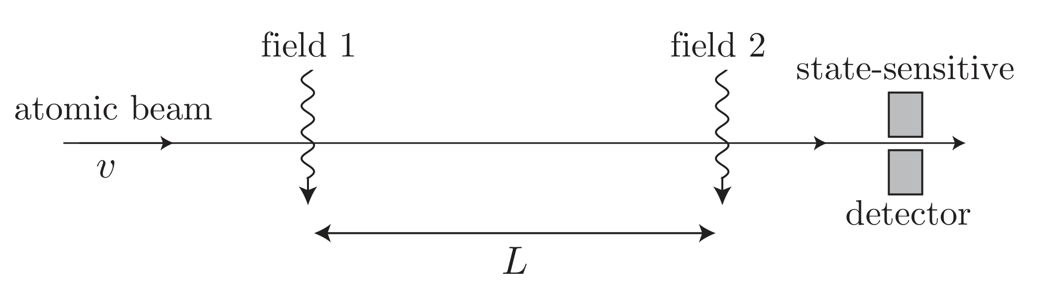
Ramsey spectroscopy is one of the most powerful techniques for precision frequency measurements in quantum optics. It is the basic operating principle behind atomic clocks. It rests on a simple yet profound idea: coherent control of a two-level system using two separated pulses.
Ramsey Spectroscopy
Rotating Frame Hamiltonian
Consider a two-level system interacting with a monochromatic field
H = 1 2 ℏ ω 0 σ z + ℏ Ω 0 cos ( ω t + ϕ 0 ) σ x H = \frac{1}{2} \hbar \omega_0 \sigma_z +\hbar\Omega_0 \cos(\omega t+\phi_0) \sigma_x
H = 2 1 ℏ ω 0 σ z + ℏ Ω 0 cos ( ω t + ϕ 0 ) σ x
H = 1 2 ℏ ω 0 σ z + 1 2 ℏ Ω 0 [ e i ( ω t + ϕ 0 ) + e − i ( ω t + ϕ 0 ) ] ( σ † + σ ) H=\frac{1}{2}\hbar\omega_0 \sigma_z +\frac{1}{2} \hbar\Omega_0 \left[\mathrm{e}^{\mathrm{i}(\omega t+\phi_0)} +\mathrm{e}^{-\mathrm{i}(\omega t+\phi_0)}\right] (\sigma^\dagger +\sigma)
H = 2 1 ℏ ω 0 σ z + 2 1 ℏ Ω 0 [ e i ( ω t + ϕ 0 ) + e − i ( ω t + ϕ 0 ) ] ( σ † + σ )
where σ † \sigma^\dagger σ † ∣ ↑ ⟩ ⟨ ↓ ∣ \ket{\uparrow}\bra{\downarrow} ∣ ↑ ⟩ ⟨ ↓ ∣ σ \sigma σ ∣ ↓ ⟩ ⟨ ↑ ∣ \ket{\downarrow}\bra{\uparrow} ∣ ↓ ⟩ ⟨ ↑ ∣
ω 0 → ω 0 + Ω 0 2 2 ( ω 0 + ω ) \omega_0 \to \omega_0 + \frac{\Omega_0^2}{2(\omega_0+\omega)}
ω 0 → ω 0 + 2 ( ω 0 + ω ) Ω 0 2
Typically atomic frequency ω 0 \omega_0 ω 0 2 π × 100 T H z 2\pi \times 100 \, \mathrm{THz} 2 π × 100 THz Ω 0 \Omega_0 Ω 0 2 π × 100 K H z 2\pi \times 100 \, \mathrm{KHz} 2 π × 100 KHz very very very small . It is kept only for completeness.
Hence we can remove this counter-rotating term and write
H = 1 2 ℏ [ ω 0 + Ω 0 2 2 ( ω 0 + ω ) ] σ z + 1 2 ℏ Ω 0 [ σ e i ( ω t + ϕ 0 ) + σ † e − i ( ω t + ϕ 0 ) ] H=\frac{1}{2}\hbar \left[\omega_0 + \frac{\Omega_0^2}{2(\omega_0+\omega)}\right] \sigma_z +\frac{1}{2} \hbar\Omega_0 \left[\sigma\mathrm{e}^{\mathrm{i}(\omega t+\phi_0)}+\sigma^\dagger \mathrm{e}^{-\mathrm{i}(\omega t+\phi_0)}\right]
H = 2 1 ℏ [ ω 0 + 2 ( ω 0 + ω ) Ω 0 2 ] σ z + 2 1 ℏ Ω 0 [ σ e i ( ω t + ϕ 0 ) + σ † e − i ( ω t + ϕ 0 ) ]
Defining U = e i 2 ω t σ z U = \mathrm{e}^{\frac{\mathrm{i}}{2}\omega t\sigma_z} U = e 2 i ω t σ z
H ~ = U H U † + i ℏ U ˙ U † = − 1 2 ℏ Δ σ z + 1 2 ℏ Ω 0 ( σ † e − i ϕ 0 + σ e i ϕ 0 ) \tilde{H} = U H U^\dagger + \mathrm{i}\hbar \dot{U} U^\dagger = -\frac{1}{2}\hbar\Delta \sigma_z + \frac{1}{2} \hbar \Omega_0 (\sigma^\dagger\mathrm{e}^{-\mathrm{i}\phi_0} + \sigma\mathrm{e}^{\mathrm{i}\phi_0})
H ~ = U H U † + i ℏ U ˙ U † = − 2 1 ℏΔ σ z + 2 1 ℏ Ω 0 ( σ † e − i ϕ 0 + σ e i ϕ 0 )
where Δ = ω − [ ω 0 + Ω 0 2 2 ( ω 0 + ω ) ] \Delta = \omega - \left[\omega_0 + \frac{\Omega_0^2}{2(\omega_0+\omega)}\right] Δ = ω − [ ω 0 + 2 ( ω 0 + ω ) Ω 0 2 ]
U ~ = exp ( − i ℏ H ~ t ) = [ cos Ω t 2 + i Δ Ω sin Ω t 2 − i sin Ω t 2 Ω 0 Ω e − i ϕ 0 − i sin Ω t 2 Ω 0 Ω e i ϕ 0 cos Ω t 2 − i Δ Ω sin Ω t 2 ] \tilde{U} = \exp\left( - \frac{\mathrm{i}}{\hbar} \tilde{H} t\right) =
\begin{bmatrix}
\cos\frac{\Omega t}{2} + \mathrm{i} \frac{\Delta}{\Omega} \sin\frac{\Omega t}{2} & -\mathrm{i} \sin\frac{\Omega t}{2} \frac{\Omega_0}{\Omega} \mathrm{e}^{-\mathrm{i}\phi_0} \\
-\mathrm{i} \sin\frac{\Omega t}{2} \frac{\Omega_0}{\Omega} \mathrm{e}^{\mathrm{i}\phi_0} & \cos\frac{\Omega t}{2} - \mathrm{i} \frac{\Delta}{\Omega} \sin\frac{\Omega t}{2}
\end{bmatrix}
U ~ = exp ( − ℏ i H ~ t ) = [ cos 2 Ω t + i Ω Δ sin 2 Ω t − i sin 2 Ω t Ω Ω 0 e i ϕ 0 − i sin 2 Ω t Ω Ω 0 e − i ϕ 0 cos 2 Ω t − i Ω Δ sin 2 Ω t ]
The state of the spins
∣ ψ ~ ( t ) ⟩ = U ~ ∣ ψ ~ ( 0 ) ⟩ = U ~ ∣ ↓ ⟩ \ket{\tilde{\psi}(t)} = \tilde{U} \ket{\tilde{\psi}(0)} = \tilde{U} \ket{\downarrow}
∣ ψ ~ ( t ) ⟩ = U ~ ∣ ψ ~ ( 0 ) ⟩ = U ~ ∣ ↓ ⟩
and switching back to the lab frame (Schrödinger picture)
∣ ψ ( t ) ⟩ = e − i 2 ω t σ z ∣ ψ ~ ( t ) ⟩ = e − i 2 ω t σ z U ~ ∣ ↓ ⟩ = [ − i sin Ω t 2 Ω 0 Ω e − i ϕ 0 e − i 2 ω t e i 2 ω t ( cos Ω t 2 − i Δ Ω sin Ω t 2 ) ] \ket{\psi(t)} = \mathrm{e}^{-\frac{\mathrm{i}}{2}\omega t\sigma_z} \ket{\tilde{\psi}(t)} = \mathrm{e}^{-\frac{\mathrm{i}}{2}\omega t\sigma_z} \tilde{U} \ket{\downarrow} =
\begin{bmatrix}
-\mathrm{i} \sin\frac{\Omega t}{2} \frac{\Omega_0}{\Omega} \mathrm{e}^{-\mathrm{i}\phi_0} \mathrm{e}^{-\frac{\mathrm{i}}{2}\omega t} \\
\mathrm{e}^{\frac{\mathrm{i}}{2}\omega t} \left( \cos\frac{\Omega t}{2} - \mathrm{i} \frac{\Delta}{\Omega} \sin\frac{\Omega t}{2} \right)
\end{bmatrix}
∣ ψ ( t ) ⟩ = e − 2 i ω t σ z ∣ ψ ~ ( t ) ⟩ = e − 2 i ω t σ z U ~ ∣ ↓ ⟩ = [ − i sin 2 Ω t Ω Ω 0 e − i ϕ 0 e − 2 i ω t e 2 i ω t ( cos 2 Ω t − i Ω Δ sin 2 Ω t ) ]
Experiment
Assume the atoms start in the ground state. At t = 0 t=0 t = 0 Ω 0 \Omega_0 Ω 0 π / 2 \pi/2 π /2 Ω 0 τ = π / 2 \Omega_0 \tau = \pi/2 Ω 0 τ = π /2
Then, we let the atom undergo free evolution precession about the z-axis for a time T T T
Finally, we apply the second π / 2 \pi/2 π /2
First pulse
At time τ = π 2 Ω 0 \tau = \frac{\pi}{2\Omega_0} τ = 2 Ω 0 π
∣ ⟨ ↑ ∣ ψ ( τ ) ⟩ ∣ 2 = Ω 0 2 Ω 0 2 + Δ 2 sin 2 Ω 0 2 + Δ 2 τ 2 = Ω 0 2 Ω 2 sin 2 Ω τ 2 |\langle \uparrow | \psi(\tau)\rangle|^2= \frac{\Omega_0^2}{\Omega_0^2+\Delta^2} \sin^2\frac{\sqrt{\Omega_0^2+\Delta^2} \tau}{2} = \frac{\Omega_0^2}{\Omega^2} \sin^2\frac{\Omega \tau}{2}
∣ ⟨ ↑ ∣ ψ ( τ )⟩ ∣ 2 = Ω 0 2 + Δ 2 Ω 0 2 sin 2 2 Ω 0 2 + Δ 2 τ = Ω 2 Ω 0 2 sin 2 2 Ω τ
Free precession
The spins process freely for time T T T
H = 1 2 ℏ ω 0 σ z → H ~ = 1 2 ℏ ( ω 0 − ω ) σ z = − 1 2 ℏ Δ σ z H = \frac{1}{2} \hbar \omega_0 \sigma_z \to \tilde{H}= \frac{1}{2}\hbar (\omega_0-\omega)\sigma_z = -\frac{1}{2}\hbar\Delta \sigma_z
H = 2 1 ℏ ω 0 σ z → H ~ = 2 1 ℏ ( ω 0 − ω ) σ z = − 2 1 ℏΔ σ z
thus the evolution operator is
U ~ = exp ( − i ℏ H ~ T ) = exp ( i 2 Δ T σ z ) = [ e i 2 Δ T 0 0 e − i 2 Δ T ] \tilde{U} = \exp\left( - \frac{\mathrm{i}}{\hbar} \tilde{H} T \right) = \exp\left(\frac{\mathrm{i}}{2} \Delta T \sigma_z\right) = \begin{bmatrix}
\mathrm{e}^{\frac{\mathrm{i}}{2}\Delta T} & 0\\
0 & \mathrm{e}^{-\frac{\mathrm{i}}{2}\Delta T}
\end{bmatrix}
U ~ = exp ( − ℏ i H ~ T ) = exp ( 2 i Δ T σ z ) = [ e 2 i Δ T 0 0 e − 2 i Δ T ]
The state of the spins after the procession in the rotating frame is
∣ ψ ~ ( τ + T ) ⟩ = [ e i 2 Δ T 0 0 e − i 2 Δ T ] [ − i sin Ω t 2 Ω 0 Ω e − i ϕ 0 cos Ω t 2 − i Δ Ω sin Ω t 2 ] = [ − i sin Ω τ 2 Ω 0 Ω e − i ϕ 0 e i 2 Δ T e − i 2 Δ T ( cos Ω τ 2 − i Δ Ω sin Ω τ 2 ) ] \ket{\tilde{\psi}(\tau+T)} =
\begin{bmatrix}
\mathrm{e}^{\frac{\mathrm{i}}{2}\Delta T} & 0\\
0 & \mathrm{e}^{-\frac{\mathrm{i}}{2}\Delta T}
\end{bmatrix}
\begin{bmatrix}
-\mathrm{i} \sin\frac{\Omega t}{2} \frac{\Omega_0}{\Omega} \mathrm{e}^{-\mathrm{i}\phi_0} \\
\cos\frac{\Omega t}{2} - \mathrm{i} \frac{\Delta}{\Omega} \sin\frac{\Omega t}{2}
\end{bmatrix} =
\begin{bmatrix}
-\mathrm{i} \sin\frac{\Omega \tau}{2} \frac{\Omega_0}{\Omega} \mathrm{e}^{-\mathrm{i}\phi_0} \mathrm{e}^{\frac{\mathrm{i}}{2}\Delta T} \\
\mathrm{e}^{-\frac{\mathrm{i}}{2}\Delta T} \left( \cos\frac{\Omega \tau}{2} - \mathrm{i} \frac{\Delta}{\Omega} \sin\frac{\Omega \tau}{2} \right)
\end{bmatrix}
∣ ψ ~ ( τ + T ) ⟩ = [ e 2 i Δ T 0 0 e − 2 i Δ T ] [ − i sin 2 Ω t Ω Ω 0 e − i ϕ 0 cos 2 Ω t − i Ω Δ sin 2 Ω t ] = [ − i sin 2 Ω τ Ω Ω 0 e − i ϕ 0 e 2 i Δ T e − 2 i Δ T ( cos 2 Ω τ − i Ω Δ sin 2 Ω τ ) ]
Second pulse
The second pulse has the same duration τ \tau τ φ \varphi φ ϕ 0 \phi_0 ϕ 0 ϕ 0 + φ \phi_0 +\varphi ϕ 0 + φ
∣ ψ ~ ( 2 τ + T ) ⟩ = U ~ ∣ ψ ~ ( τ + T ) ⟩ \ket{\tilde{\psi}(2\tau +T)} = \tilde{U} \ket{\tilde{\psi}(\tau+T)}
∣ ψ ~ ( 2 τ + T ) ⟩ = U ~ ∣ ψ ~ ( τ + T ) ⟩
∣ ψ ~ ( 2 τ + T ) ⟩ = [ cos Ω τ 2 + i Δ Ω sin Ω τ 2 − i sin Ω τ 2 Ω 0 Ω e − i ( ϕ 0 + φ ) − i sin Ω τ 2 Ω 0 Ω e i ( ϕ 0 + φ ) cos Ω τ 2 − i Δ Ω sin Ω τ 2 ] [ − i sin Ω τ 2 Ω 0 Ω e − i ϕ 0 e i 2 Δ T e − i 2 Δ T ( cos Ω τ 2 − i Δ Ω sin Ω τ 2 ) ] \ket{\tilde{\psi}(2\tau +T)} = \begin{bmatrix}
\cos\frac{\Omega \tau}{2} + \mathrm{i} \frac{\Delta}{\Omega} \sin\frac{\Omega \tau}{2} & -\mathrm{i} \sin\frac{\Omega \tau}{2} \frac{\Omega_0}{\Omega} \mathrm{e}^{-\mathrm{i}(\phi_0+\varphi)} \\
-\mathrm{i} \sin\frac{\Omega \tau}{2} \frac{\Omega_0}{\Omega} \mathrm{e}^{\mathrm{i}(\phi_0+\varphi)} & \cos\frac{\Omega \tau}{2} - \mathrm{i} \frac{\Delta}{\Omega} \sin\frac{\Omega \tau}{2}
\end{bmatrix} \begin{bmatrix}
-\mathrm{i} \sin\frac{\Omega \tau}{2} \frac{\Omega_0}{\Omega} \mathrm{e}^{-\mathrm{i}\phi_0} \mathrm{e}^{\frac{\mathrm{i}}{2}\Delta T} \\
\mathrm{e}^{-\frac{\mathrm{i}}{2}\Delta T} \left( \cos\frac{\Omega \tau}{2} - \mathrm{i} \frac{\Delta}{\Omega} \sin\frac{\Omega \tau}{2} \right)
\end{bmatrix}
∣ ψ ~ ( 2 τ + T ) ⟩ = [ cos 2 Ω τ + i Ω Δ sin 2 Ω τ − i sin 2 Ω τ Ω Ω 0 e i ( ϕ 0 + φ ) − i sin 2 Ω τ Ω Ω 0 e − i ( ϕ 0 + φ ) cos 2 Ω τ − i Ω Δ sin 2 Ω τ ] [ − i sin 2 Ω τ Ω Ω 0 e − i ϕ 0 e 2 i Δ T e − 2 i Δ T ( cos 2 Ω τ − i Ω Δ sin 2 Ω τ ) ]
after some horrible calculations, we finally obtain
∣ ψ ~ ( 2 τ + T ) ⟩ = [ − i sin Ω τ 2 Ω 0 Ω e − i ϕ 0 [ e i 2 Δ T ( cos Ω τ 2 + i Δ Ω sin Ω τ 2 ) + e − i φ e − i 2 Δ T ( cos Ω τ 2 − i Δ Ω sin Ω τ 2 ) ] − sin 2 Ω τ 2 ( Ω 0 Ω ) 2 e i φ e i 2 Δ T + e − i 2 Δ T ( cos Ω τ 2 − i Δ Ω sin Ω τ 2 ) 2 ] \ket{\tilde{\psi}(2\tau + T)} =
\begin{bmatrix}
-\mathrm{i} \sin\frac{\Omega \tau}{2} \frac{\Omega_0}{\Omega}\mathrm{e}^{-\mathrm{i}\phi_0} \left[\mathrm{e}^{\frac{\mathrm{i}}{2}\Delta T}\left(\cos\frac{\Omega \tau}{2} + \mathrm{i} \frac{\Delta}{\Omega} \sin\frac{\Omega \tau}{2}\right) + \mathrm{e}^{-\mathrm{i}\varphi}\mathrm{e}^{-\frac{\mathrm{i}}{2}\Delta T}\left( \cos\frac{\Omega \tau}{2} - \mathrm{i} \frac{\Delta}{\Omega} \sin\frac{\Omega \tau}{2} \right)\right]
\\
- \sin^2 \frac{\Omega \tau}{2} \left(\frac{\Omega_0}{\Omega}\right)^2 \mathrm{e}^{\mathrm{i}\varphi} \mathrm{e}^{\frac{\mathrm{i}}{2}\Delta T} + \mathrm{e}^{-\frac{\mathrm{i}}{2}\Delta T} \left( \cos\frac{\Omega \tau}{2} - \mathrm{i} \frac{\Delta}{\Omega} \sin\frac{\Omega \tau}{2} \right)^2
\end{bmatrix}
∣ ψ ~ ( 2 τ + T ) ⟩ = [ − i sin 2 Ω τ Ω Ω 0 e − i ϕ 0 [ e 2 i Δ T ( cos 2 Ω τ + i Ω Δ sin 2 Ω τ ) + e − i φ e − 2 i Δ T ( cos 2 Ω τ − i Ω Δ sin 2 Ω τ ) ] − sin 2 2 Ω τ ( Ω Ω 0 ) 2 e i φ e 2 i Δ T + e − 2 i Δ T ( cos 2 Ω τ − i Ω Δ sin 2 Ω τ ) 2 ]
Switching back to the lab frame just add an global dynamical phase to each component
∣ ψ ( 2 τ + T ) ⟩ = [ − i sin Ω τ 2 Ω 0 Ω e − i ϕ 0 e − i 2 ω ( 2 τ + T ) [ e i 2 Δ T ( cos Ω τ 2 + i Δ Ω sin Ω τ 2 ) + e − i φ e − i 2 Δ T ( cos Ω τ 2 − i Δ Ω sin Ω τ 2 ) ] − sin 2 Ω τ 2 ( Ω 0 Ω ) 2 e i φ e i 2 Δ T e − i 2 ω ( 2 τ + T ) + e − i 2 Δ T e i 2 ω ( 2 τ + T ) ( cos Ω τ 2 − i Δ Ω sin Ω τ 2 ) 2 ] \ket{\psi(2\tau + T)} =
\begin{bmatrix}
-\mathrm{i} \sin\frac{\Omega \tau}{2} \frac{\Omega_0}{\Omega}\mathrm{e}^{-\mathrm{i}\phi_0} \mathrm{e}^{-\frac{\mathrm{i}}{2} \omega (2\tau+T)}\left[\mathrm{e}^{\frac{\mathrm{i}}{2}\Delta T}\left(\cos\frac{\Omega \tau}{2} + \mathrm{i} \frac{\Delta}{\Omega} \sin\frac{\Omega \tau}{2}\right) + \mathrm{e}^{-\mathrm{i}\varphi}\mathrm{e}^{-\frac{\mathrm{i}}{2}\Delta T}\left( \cos\frac{\Omega \tau}{2} - \mathrm{i} \frac{\Delta}{\Omega} \sin\frac{\Omega \tau}{2} \right)\right]
\\
- \sin^2 \frac{\Omega \tau}{2} \left(\frac{\Omega_0}{\Omega}\right)^2 \mathrm{e}^{\mathrm{i}\varphi} \mathrm{e}^{\frac{\mathrm{i}}{2}\Delta T}\mathrm{e}^{-\frac{\mathrm{i}}{2} \omega (2\tau+T)} + \mathrm{e}^{-\frac{\mathrm{i}}{2}\Delta T} \mathrm{e}^{\frac{\mathrm{i}}{2} \omega (2\tau+T)}\left( \cos\frac{\Omega \tau}{2} - \mathrm{i} \frac{\Delta}{\Omega} \sin\frac{\Omega \tau}{2} \right)^2
\end{bmatrix}
∣ ψ ( 2 τ + T ) ⟩ = [ − i sin 2 Ω τ Ω Ω 0 e − i ϕ 0 e − 2 i ω ( 2 τ + T ) [ e 2 i Δ T ( cos 2 Ω τ + i Ω Δ sin 2 Ω τ ) + e − i φ e − 2 i Δ T ( cos 2 Ω τ − i Ω Δ sin 2 Ω τ ) ] − sin 2 2 Ω τ ( Ω Ω 0 ) 2 e i φ e 2 i Δ T e − 2 i ω ( 2 τ + T ) + e − 2 i Δ T e 2 i ω ( 2 τ + T ) ( cos 2 Ω τ − i Ω Δ sin 2 Ω τ ) 2 ]
It does not depend on ϕ 0 \phi_0 ϕ 0 φ \varphi φ ϕ 0 \phi_0 ϕ 0
The probability is
P ↑ = ∣ ⟨ ↑ ∣ ψ ( 2 τ + T ) ⟩ ∣ 2 = 4 Ω 0 2 Ω 2 sin 2 Ω τ 2 ∣ cos Ω τ 2 cos ( Δ T 2 − φ 2 ) − Δ Ω sin Ω τ 2 sin ( Δ T 2 − φ 2 ) ∣ 2 P_\uparrow = |\langle \uparrow | \psi(2\tau+T)\rangle|^2= \frac{4\Omega_0^2}{\Omega^2} \sin^2\frac{\Omega \tau}{2} \left| \cos \frac{\Omega \tau}{2} \cos\left(\frac{\Delta T}{2} - \frac{\varphi}{2}\right) -\frac{\Delta}{\Omega}\sin \frac{\Omega \tau}{2} \sin\left(\frac{\Delta T}{2} - \frac{\varphi}{2}\right) \right|^2
P ↑ = ∣ ⟨ ↑ ∣ ψ ( 2 τ + T )⟩ ∣ 2 = Ω 2 4 Ω 0 2 sin 2 2 Ω τ cos 2 Ω τ cos ( 2 Δ T − 2 φ ) − Ω Δ sin 2 Ω τ sin ( 2 Δ T − 2 φ ) 2
Again, substitute τ = π 2 Ω 0 \tau = \frac{\pi}{2\Omega_0} τ = 2 Ω 0 π
P ↑ = 4 Ω 0 2 Ω 2 sin 2 ( Ω Ω 0 π 4 ) ∣ cos ( Ω Ω 0 π 4 ) cos ( Δ T 2 − φ 2 ) − Δ Ω sin ( Ω Ω 0 π 4 ) sin ( Δ T 2 − φ 2 ) ∣ 2 P_\uparrow = \frac{4\Omega_0^2}{\Omega^2} \sin^2 \left(\frac{\Omega}{\Omega_0}\frac{\pi}{4}\right) \left| \cos \left(\frac{\Omega}{\Omega_0}\frac{\pi}{4}\right) \cos\left(\frac{\Delta T}{2} - \frac{\varphi}{2}\right) -\frac{\Delta}{\Omega}\sin \left(\frac{\Omega}{\Omega_0}\frac{\pi}{4}\right) \sin\left(\frac{\Delta T}{2} - \frac{\varphi}{2}\right) \right|^2
P ↑ = Ω 2 4 Ω 0 2 sin 2 ( Ω 0 Ω 4 π ) cos ( Ω 0 Ω 4 π ) cos ( 2 Δ T − 2 φ ) − Ω Δ sin ( Ω 0 Ω 4 π ) sin ( 2 Δ T − 2 φ ) 2
Near resonance, Δ ≪ Ω \Delta \ll \Omega Δ ≪ Ω
P ↑ = Ω 0 2 Ω 2 sin 2 ( Ω Ω 0 π 4 ) cos 2 ( Δ T 2 − φ 2 ) P_\uparrow = \frac{\Omega_0^2}{\Omega^2} \sin^2 \left(\frac{\Omega}{\Omega_0}\frac{\pi}{4}\right)\cos^2\left(\frac{\Delta T}{2} - \frac{\varphi}{2}\right)
P ↑ = Ω 2 Ω 0 2 sin 2 ( Ω 0 Ω 4 π ) cos 2 ( 2 Δ T − 2 φ )
It yields a fringe pattern in detuning Δ \Delta Δ
As shown in the figure, the laser frequency ω \omega ω
ω fringe = 2 π T \omega_\text{fringe} = \frac{2\pi}{T}
ω fringe = T 2 π
while the overall envelope of the curve follows the Rabi lineshape
P ↑ envelope = Ω 0 2 Ω 2 sin 2 ( Ω Ω 0 π 4 ) = Ω 0 2 Ω 0 2 + Δ 2 sin 2 ( Ω 0 2 + Δ 2 Ω 0 π 4 ) P_\uparrow^\text{envelope}=\frac{\Omega_0^2}{\Omega^2} \sin^2 \left(\frac{\Omega}{\Omega_0}\frac{\pi}{4}\right)=\frac{\Omega_0^2}{\Omega_0^2+\Delta^2} \sin^2 \left(\frac{\sqrt{\Omega_0^2+\Delta^2}}{\Omega_0}\frac{\pi}{4}\right)
P ↑ envelope = Ω 2 Ω 0 2 sin 2 ( Ω 0 Ω 4 π ) = Ω 0 2 + Δ 2 Ω 0 2 sin 2 ( Ω 0 Ω 0 2 + Δ 2 4 π )